
Tags and keywords
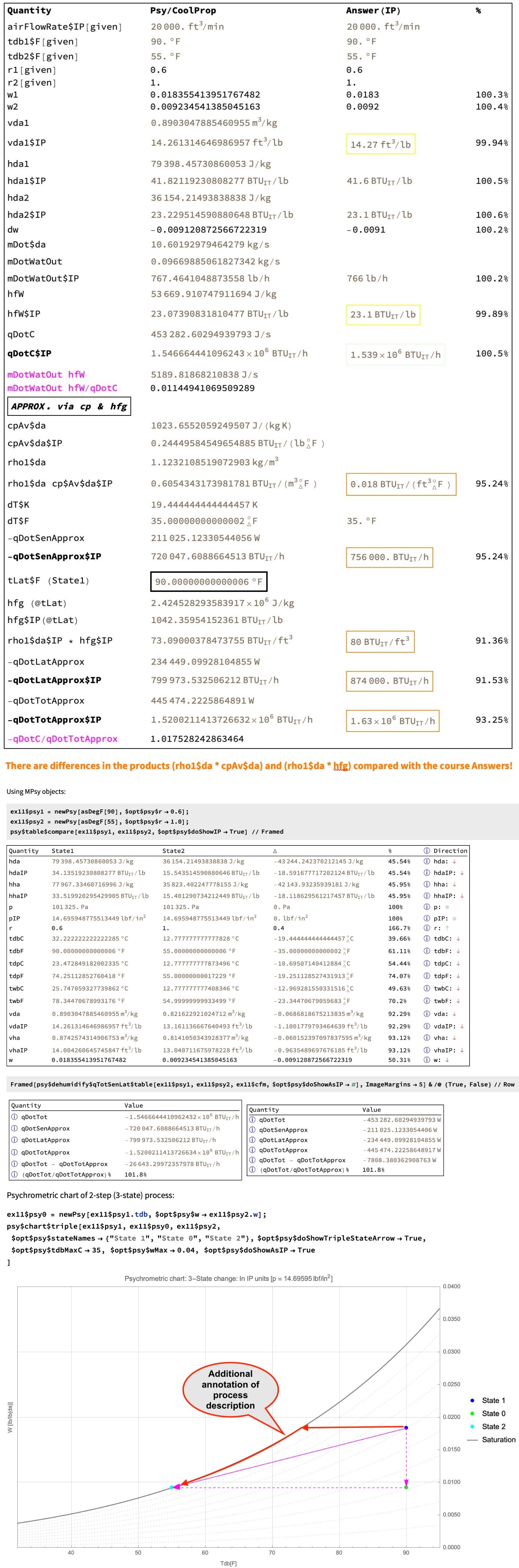
The course PDF Answers (where available) from the worked example problem are given in the 3rd column in the custom table at the top of the slide image in IP units. Note how that table shows both the accurately computed total heat exchange rate (denoted 'Qc' in the worked course solutions), and the approximate values for the sensible and latent heat contributions.
In the more accurate total heat transfer 'qDotTot' calculation (which in the Psy library convention has the opposite sign to 'Qc'), the specific enthalpy of the condensed water is taken at the dry bulb temperature of State2 (at the final saturation point). The value from CoolProp thus taken agrees well with the provided course Answer value.
It is interesting to note that the product mDotWatOut * hfW of the mass flow rate of the water and the specific enthalpy of the liquid water is only about 1% of the total heat exchange rate, and this term is often dropped from approximate methods.
The course PDF says:
It is assumed that this means that it is considered pure sensible cooling (at the humidity ratio 'w1' of State1), then as condensation along the saturation curve (with change of both humidity ratio 'w' and dry bulb temperature 'tdb' until the dry bulb temperature and target humidity ratio of State2 are reached), as shown on the chart as an additional annotation (in red). Note that this description does not refer to approximate treatment as a 2-step pure latent then pure sensible process, just to the depiction on a chart.
If the problem is treated as a 2-step process, a condensation with release of latent heat followed by sensible cooling, the latent heat of vaporisation 'hfg' of the water can be estimated at the dry bulb temperature of the initial State1, and the specific heat capacity of the dry air can be estimated using an average of the values at the dry bulb temperatures of State1 and the final State2 and at the humidity ratio of State2 (see the tables in the Postscript below for their sensitivities).
It is assumed that the given volumetric air flow rate is that of the humid air mixture. Thus, the mass flow rate per dry air mDot$da is determined via the volume per dry air vda1$da (equals 1/rho1$da) at entry State1.
When handled by the Webel MPsy class, we have 2 objects representing the before (State1) and after (State2) states.
The 2nd table shows the differences between State1 (initial) and State2 (final), as well as indicating the change in each main psychrometric variables, and the "direction" of change.
There is a dedicated Psy library function for calculating and displaying the more accurately computed 'qDotTot', and the approximate 'qDotSenApprox', and 'qDotLatApprox', as shown in the 3rd table. It can been seen that the total of the approximate contributions is within about 1% of the more accurate total heat exchange rate calculation 'qDotTot', which gives some confidence in the choices of the average specific heat capacity of dry air 'cpAv$da' and the latent heat of vaporisation of the water 'hfg' used here.
The calculated approximate sensible heat rate 'qDotSenApprox' only within about 5% of the Answer provided in the course, and the approximate latent heat rate 'qDotLatApprox' disagrees by about 10% with the Answer provided in the course. Presumably their average specific heat capacity per dry air 'cpAv$da' and latent heat of vaporisation 'hfg' is not as accurate. If 'hfg' is chosen at the final State2 (55 °F) instead of at the initial State1 (90 °F) the agreement with the provided course Answers is slightly better.
The Webel Psy package adopts the following convention:
Energy has been transferred as sensible heat FROM the humid air TO the cold sink, so 'qDotSenApprox' is considered -ve.
Energy has been transferred as released latent heat of vaporisation FROM the humid air TO the cold sink, so 'qDotLatApprox' is considered -ve.
In the case of air-conditioning with a heat exchanger cooling coil with tubes containing refrigerant (colder than the air), the outer surface of the tubes (and any fins) may be colder than the dew point temperature of the air. (The refrigerant itself and the inner tube surface will be colder than the outer surface due to any thermal resistance of the tube.) Both the sensible heat and the latent heat will be primarily carried away by the fin/tube surfaces (and will heat the refrigerant), and are lost to the humid air.
The psychrometric chart function shows State1, the intermediate "State0" (when modelled as a 2-step process) and State2, as well as an arrow indicating the changes between State1 (initial) and State2 (final), and dashed arrows to and from "State0" for the 2-step approach.
Postscript concerning the variation of values between states and the need for averages
The following values are according to CoolProp:
The variation in the latent heat of vaporisation of water 'hfg' between the temperature of State1 and the temperature at State2 (recall it was estimated at the temperature 90 °F of State1 in the calculation of the 'qDotLatApprox'):
90 °F	hfg = 2.424528293583917 10^6 J/kg
55 °F	hfg = 2.470610630477806 10^6 J/kg
90 °F	w = 0.009234541385045163` 	cp$da = 1023.9501474814153 J / (kg K)
55 °F	w = 0.009234541385045163` 	cp$da = 1023.3602643684859 J /(kg K)
These variations are significant enough to require at least some averaging (and preferably numerical integration) when using approximate calculation of the sensible and latent heat exchange rate contributions.
The range of the density per dry air 'rho$da' between initial State1 and intermediate State0 is:
90 °F	w = 0.018355413951767482` 	rho$da = 1.1232108519072903 kg/m^3
90 °F	w = 0.009234541385045163` 	rho$da = 1.1393850533713705 kg/m^3
The range of the density per dry air 'rho$da' between intermediate State0 and final State2 is:
90 °F	w = 0.009234541385045163` 	rho$da = 1.13938505337137 kg/m^3
55 °F	w = 0.009234541385045163` 	rho$da = 1.21710333829638 kg/m^3
Note that this implies that - for constant mass flow rate per dry air - the volume per dry air can vary (and indeeed does for the process shown).